A Kick in the Discovery

This article is meant to be an intuitive introduction to metric spaces. We aim to motivate the concept of a metric space and some fundamental theorems about them, and have as much fun as we can along the way.

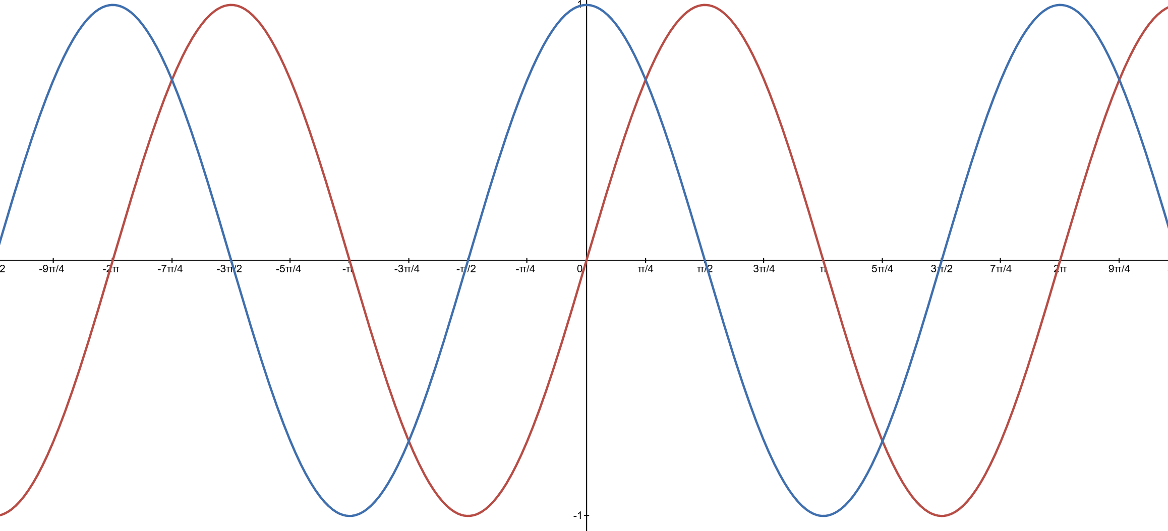
To begin, let me ask you a question: What is the distance between sine and cosine? I can hear you thinking, “What does that mean?” Which is a good question! What does it mean? When I hear this question, I think of taking their difference $|\sin(x) – \cos(x)|,$ but of course, at different $x$ values their difference is different! However, if you wanted to give one number as the answer what might you say?

Keep this question in mind as we begin our discussion of metric spaces. I think it’s a great one! P.S. There is more than one possible answer!

---

The key takeaways of this article are, hopefully, (1) you’ll have an intuition for the axioms of a metric space so that way you no longer need to memorize them since you’ll simply understand them, (2) you’ll have a few examples of usefull and common metric spaces, (3) you’ll understand what open sets and closed sets are along with some understanding of how to work with them.

Table of Contents

1. Motivation – What is distance?
   1. Some properties of distance
2. Open Sets
   1. What is B(𝟎,1) in the metric space (ℝ2,dE)?
   2. What is B(𝟎,1) in the metric space (ℝ2,dM)?
   3. What is B(𝟎,1) in the metric space (ℝ2,d∞)?
   4. What are some open sets in the metric space ([0,1],dE)?
3. Closed Sets
4. Intersections and Unions of Open and Closed Sets
   1. Arbitrary Unions/Intersections of Open Sets
   2. Arbitrary Unions/Intersections of Closed Sets
5. Final Remarks

Motivation – What is distance?

Here’s the deal: a metric space is a set with `added structure’.¹ In our case, the added structure is the notion of distance between points. So, given a set, $X$ we can calculate the distance between $x\in X$ and $y\in X$ and denote it $d(x,y).$

More precisely and more mathematically, a metric space is a pair $(X,d),$ where $X$ is a set with a function $d:X\times X \rightarrow \R$ that we can think of as taking in pairs of elements from $X$ and outputting a real number that equals the distance between $x,y\in X.$ But, in order for $d$ to be considered a distance function, it must satisfy certain axioms or rules.

Which begs the question: What properties should $d:X\times X \rightarrow \R$ satisfy to be a bona fide distance function? Let’s try to make a list of properties that we think are crucial to include as axioms! However, I recommend you try this first on your own! You don’t need to get the ‘correct’ answer; you just need to engage your brain with the material! Plus, it might be fun! You’ll be inventing new mathematics! As motivation, think about the properties that distance in $\R,\;\R^2,$ and $\R^3$ satisfy in everyday life.

Some properties of distance

(1) Well, right off the bat, the distance between distinct points $x,y\in X$ should be positive, i.e., it should be that $d(x,y)> 0$ for all distinct points $x,y\in X.$

(2) The distance between $x$ and itself should be zero. Moreover, the distance between $x$ and $y$ equals zero if and only if they are the same point:$d(x,y)= 0 \iff x=y.$

(3) Next, how should the distance from $x$ and $y$ compare to the distance from $y$ to $x?$ We’d like them to be equal: $d(x,y) = d(y,x)$ for all $x,y\in X.$

(4) There is one more property that we’d like our distance function to satisfy. It’s perhaps the least intuitive axiom, at first at least. We want to capture what is called the triangle inequality. Here’s the idea: imagine starting a journey at point $s$ and ending at a point $e.$ We know, intuitively, that it’s a shorter distance to go directly from $s$ to $e.$ In particular, stopping at any other point $p$ along the way will only increase the distance we travel to reach point $e.$

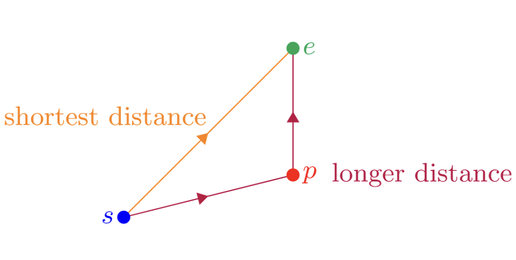
This is captured in the previous image and by the following expression:

Using the standard letters we will use throughout the article: $x,y,$ and $z,$

As it turns out, mathematicians think that these four points are the most crucial aspects of a distance function. We require nothing more out of $d.$

Altogether, we have argued for the following definition of a metric space.

Definition 1 (Metric Space): Let $X$ be a set and $d:X\times X \rightarrow \R$ be a map. We call $(X,d)$ a metric space if $d$ satisfies the following axioms,

1. (Non-Negative) $d(x,y)\geq 0$ for all $x,y\in X;$
2. (Zero iff Same Point) $d(x,y)= 0 \iff x=y;$
3. (Symmetric) $d(x,y) = d(y,x)$ for all $x,y\in X;$ and
4. (Triangle Inequality) $d(x,z) \leq d(x,y)+d(y,z)$ for all $x,y,z\in X.$

We call the map $d$ a metric if conditions (1.)-(4.) are satisfied.

Of course, with any new definition, we should see a few examples. Cool!

Example $(\R^n,d_E)$ The Euclidean Metric: (Click in the Discovery)

Let’s begin with the real line $\R.$ Intuitively, you might suggest that the distance between, say, $10$ and $29$ should be equal to $19,$ so that $d_E(10,29) = 19$. Or, that the distance between $2$ and $3$ should be equal to $1,$ so that $d_E(2,3)=1.$ Indeed, this is the intuition for the metric $d_E(x,y) = |x-y|,$ where the E stands for Euclidean. We can see that (1), (2), and (3) in Definition 1 are satisfied immediately; however, (4) is trickier. But if you’ve taken real analysis, then you’ll know that $|x-z| \leq |x-y|+|y-z|$ for all $x,y,z\in \R.$ If not, see here.

---

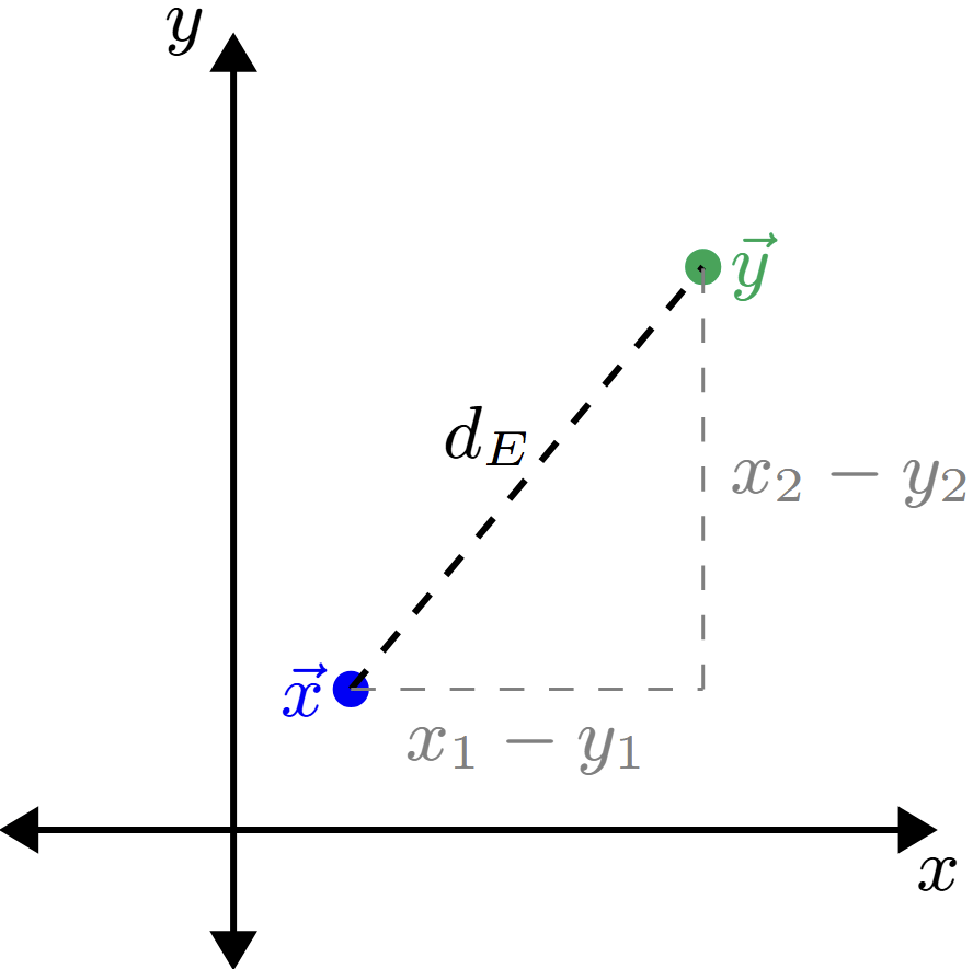
We can continue to the plane $\R^2.$ The metric we choose here is the one you are likely familiar with. It’s based on the Pythagorean theorem, which is funny when you think about it. We call the statement the Pythagorean theorem because it’s a theorem. We needed to establish it with proof, but now we are taking it as an axiom! How cool! Anyway, I digress…

Going back to defining the metric, let $x = \langle x_1,x_2 \rangle\in \R^2$ and $y = \langle y_1,y_2 \rangle\in \R^2$ be two points in the plane. Note that we are using angled brackets $\langle \cdot ,\cdot \rangle$ to denote a vector so that we don’t confuse a vector in $\R^2$ and an open interval in $\R.$ Then, we define the metric $d_E$ by,

$$d_E(x,y) := \sqrt{(x_1-y_1)^2 +(x_2-y_2)^2}.$$

We can see again that (1), (2), and (3) are satisfied, and, as will be the case most of the time, it’s more challenging to see if this notion of distance satisfies the triangle inequality. I challenge you to show that it does. However, for our purposes, we will be satisfied to say that this is a geometric fact.

The two metrics are called the Euclidean metrics on $\R$ and $\R^2.$ We can further generalize using the Pythagorean theorem as motivation to $\R^n.$ With $x = \langle x_1,x_2 ,\cdots x_n\rangle\in \R^n$ and $y = \langle y_1,y_2 ,\cdots, y_n\rangle\in \R^n$ we define the following metric,

$$d_E(x,y) = \sqrt{\sum_{k=1}^n(x_k-y_k)^2 }.$$

Example $(\R^n, d_M)$ The Manhattan Metric: (Click in the Discovery)

Consider the plane $\R^2.$ There are other metrics we can define on the plane besides the Euclidean metric. For instance, imagine if we could only move left/right and up/down. That is, we cannot move diagonally. It’s as if we are forced to move along city streets in a city grid. Then, the distance between two points would be calculated using the following metric. For $x = \langle x_1,x_2 \rangle\in \R^2$ and $y = \langle y_1,y_2 \rangle\in \R^2$ we have

$$d_M(x,y) = |x_1-y_1| +|x_2-y_2|.$$

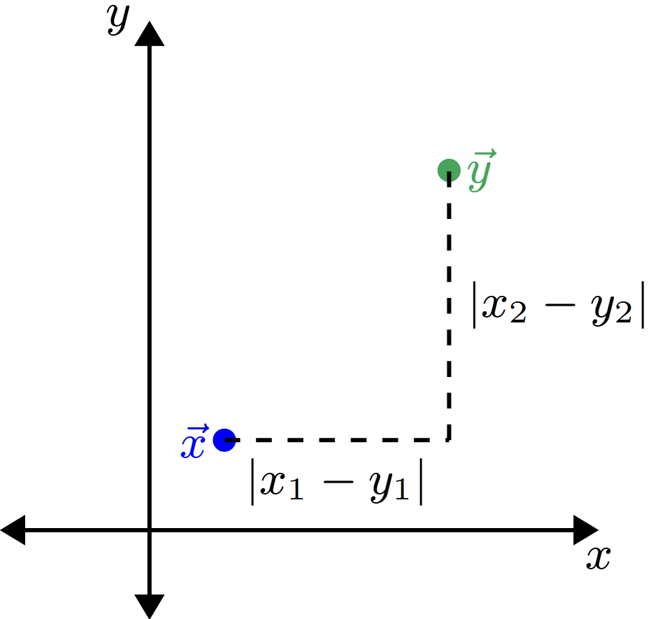
This is indeed a metric. We can see again that (1), (2), and (3) are satisfied in Definition 1, and the fact that the triangle inequality is satisfied follows from the standard triangle inequality for absolute values $|\cdot |.$

We can also generalize this metric to $\R^n.$ More precisely, let $x = \langle x_1,x_2 ,\cdots x_n\rangle\in \R^n$ and $y = \langle y_1,y_2 ,\cdots, y_n\rangle\in \R^n$ we define the following metric,

$$d_M(x,y) = \sum_{k=1}^n|x_k-y_k|.$$

Example $(\R^n,d_{\infty})$ The Infinity Metric: (Click in the Discovery)

This is the last metric we will put on $\R^n.$

First, consider the plane $\R^2.$ In this case, given two points $x = \langle x_1,x_2 \rangle\in \R^2$ and $y = \langle y_1,y_2 \rangle\in \R^2,$ we first determine how separated $x$ and $y$ are along the $x$-axis, that is, we calculate $|x_1-y_1|.$ Then, we determine how separated along the $y$ -axis $x$ and $y$ are, that is, we calculate $|x_2-y_2|.$ Then, we simply take the maximum of the two computations to be the distance,

$$d_{\infty}(x,y) = \max{\big\{|x_1-y_1|\,,\,|x_2-y_2|\big\}}.$$

We can see yet again that (1), (2), and (3) are satisfied. However, again, it’s a little more challenging to see if this notion of distance satisfies the triangle inequality. Here’s the idea: Let $x = \langle x_1,x_2 \rangle\in \R^2,$ $y = \langle y_1,y_2 \rangle\in \R^2,$ and $z = \langle z_1,z_2 \rangle\in \R^2.$ Then,

$$|x_1-z_1| \leq |x_1-y_1|+|y_1-z_1| \leq \max{\big\{|x_1-y_1|\,,\,|x_2-y_2|\big\}} + \max{\big\{|y_1-z_1|\,,\,|y_2-z_2|\big \}}$$

$$\leq d_{\infty}(x,y) + d_{\infty}(y,z)\qquad\;$$

Likewise, $|x_2-z_2|\leq d_{\infty}(x,y) + d_{\infty}(y,z).$ Consequently, $\max{\{|x_1-z_1|\,,\,|x_2-z_2| \}}\leq d_{\infty}(x,y) + d_{\infty}(y,z).$ This is our desired result $d_{\infty}(x,z)\leq d_{\infty}(x,y) + d_{\infty}(y,z).$

We can further generalize $d_{\infty}$ to $\R^n.$ Let $x = \langle x_1,x_2 ,\cdots x_n\rangle\in \R^n$ and $y = \langle y_1,y_2 ,\cdots, y_n\rangle\in \R^n$ we define the following metric,

$$d_{\infty}(x,y) =\max{\Big\{|x_k-y_k|\;:\;1\leq k\leq n\Big\}}.$$

The previous three metric spaces are all on the same set, $\R^n.$ However, the utility of metric spaces is that we can also consider other sets that may be less intuitive. In this next example, we will give one possible answer to the question we asked at the beginning.

Example $(\mathcal{C}([0,1]),d)$: (Click in the Discovery)

Recall the question: What is the distance between sine and cosine? Well, it’s time to answer! For most practical purposes, we will consider the distance between functions on a closed, bounded interval. In this case, the distance between sine and cosine over the closed unit interval $[0,1].$ Thus, we are now asking: What is the distance between the sine function and the cosine function over the interval $[0,1]$? We will change the period of sine and cosine and consider $\sin{(2\pi x)}$ and $\cos{(2\pi x)}.$

---

You might have come up with something like the following: Maybe we should fix some special $x_0\in [0,1]$ and look at the difference $|\sin{(2\pi x_0)}-\cos{(2\pi x_0)}|.$ However, how would we choose the particular $x_0$ value? However, this is not a great choice since if we happened to chose $x_0=\frac{1}{8}$ then $\sin{(\pi /4)} = \cos{(\pi /4)}$ so that their distance is zero, which contradicts point (2).

Ok, new plan… maybe we choose the value that maximizes the difference between them. That is, we say that the distance between $\sin{(2\pi x)}$ and $\cos{(2\pi x)}$ equals $\sup{\left\{|\sin{(2\pi x)}-\cos{(2\pi x)}|\;:\;x\in [0,1]\right\}}.$ (see the footnote for a reminder on what the supremum is)² Indeed, this is one way we can choose to define the distance between sine and cosine. In fact, we can use this to define the distance between any two continuous functions on the closed unit interval!

Let’s see how.

The pair $(\mathcal{C}([0,1]),d)$ is a metric space where, $\mathcal{C}([0,1])$ is the set of continuous functions $f:[0,1]\rightarrow \R$ and $d$ is the metric given by

$$d(f,g)=\sup{\left\{|f(x)-g(x)|\;:\;x\in [0,1]\right\}}\qquad \mathrm{for}\;\mathrm{all}\;f,g\in \mathcal{C}([0,1]).$$

Let’s show that this is indeed a metric. I leave it to you to prove that $d$ satisfies (1), (2). and (3); we will show that 𝑑 satisfies the triangle inequality below. But try it on your own first!

Proof: Let $f,g,h\in \mathcal{C}([0,1])$ be continuous functions. We aim to show that $d(f,h)\leq d(f,g)+d(g,h).$ First, note that $|f(x)-h(x)|$ is a continuous function on $[0,1],$ which is a closed and bounded interval. Thus, by the extreme value theorem, there is some $x_0\in [0,1]$ so that $|f(x)-h(x)|$ attains its maximum (or supremum). More preicely, $|f(x)-h(x)|\leq |f(x_0)-h(x_0)|$ for all $x\in [0,1].$ Thus,

$$d(f,h) = |f(x_0)-h(x_0)| \leq |f(x_0)-g(x_0)| + |g(x_0)-h(x_0)|$$

by the triangle inequality on absolute values. However, $|f(x)-g(x)|$ and $|g(x)-h(x)|$ are also continuous on a closed and bounded interval. It follows by the extreme value theorem that $|f(x)-g(x)| \leq |f(x_1)-g(x_1)| = d(f,g)$ and $|g(x)-h(x)| \leq |g(x_2)-h(x_2)| = d(g,h)$ for $x_1,x_2\in [0,1].$ Consequently, $|f(x_0)-g(x_0)| + |g(x_0)-h(x_0)| \leq d(f,g) + d(g,h).$ Hence,

$$d(f,h) \leq d(f,g) + d(g,h).$$

Thus concluding the proof.

Now we can give an answer to our starting question: The distance between sine and cosine on $[0,1]$ equals $\sqrt{2}.$³

There is one last metric that we want to mention. Before we do, you might ask, “Given any set $X,$ can we upgrade it to a metric space?” The answer is affirmative and is given by the so-called trivial metric, which exists for all sets.

Example (The Trivial Metric): (Click in the Discovery)

Let $X$ be any set. We define the following metric, $d:X\times X\rightarrow \R$

$$d(x,y) = \begin{cases} 1, \qquad \mathrm{if}\;\; x\neq y \\ 0, \qquad \mathrm{if}\;\; x= y. \end{cases}$$

Again, $(X,d)$ satisfies all the axioms of a metric space. Although proving the triangle inequality case by case is tedious.

Open Sets

Recall that open intervals in $\R$ are of the form $(a,b)$ for $a<b\in \R$ and that closed intervals in $\R$ are of the form $[a,b]$ for $a<b\in \R.$ What differentiates these two sets from one another? This is a loaded question with no obvious correct answer. It turns out that the key feature that we want to hone in on is the fact that any point $x\in (a,b)$ has another smaller open interval centered at $x$ that is contained in $(a,b).$ That is, for any $x\in (a,b),$ there exists some $\varepsilon>0$ such that $(x-\varepsilon\,,x+\varepsilon) \subset (a,b).$ For instance, consider the open unit interval $(0,1)$ and the point $0.25\in (0,1).$ We see that $(0.25 – 0.01 \;,\; 0.25 +0.01)= \left(0.24\;,\;0.26 \right) \subset (0,1).$ However, in a non-open interval, such as $[a,b]$ or $[a,b)$ the endpoint $a$ doesn’t have this property. This is because $(a-\varepsilon,a+\varepsilon)$ is not contained in $[a,b]$ for any $\varepsilon>0.$

Thus, we call $(a,b)\subset \R$ an open interval because no matter what $x\in (a,b),$ we can always find a small enough $\varepsilon>0$ such that $(x-\varepsilon\,,x+\varepsilon) \subset (a,b).$

We take this property and raise it to general metric spaces. However, let’s first define an open ball and a closed ball. These are the generalizations of the two intervals: $(x-\varepsilon \,,x+\varepsilon)$ and $[x-\varepsilon\,,x+\varepsilon].$ But we will replace $\varepsilon>0$ with $r>0$ because we will think of it as a radius.

Definition 2 (Open and Closed Balls): Let $(X,d)$ be a metric space and let $x\in X$ and $r>0.$ We define an open ball in $(X,d)$ to be the set

$$B(x,r) := \{y\in X\;:\;d(x,y)<r \}.$$

Next, we define the closed ball to be the set,

$$\mathrm{cl}{B}(x,r) := \{y\in X\;:\;d(x,y)\leq r \}.$$

In both cases, we call $x\in X$ the center of the ball and $r>0$ the radius.

Remark 1: In $(\R,d_E),$ an open ball has the form $B(x,r)=(x-r\,,x+r)$ and a closed ball has the form $\mathrm{cl}B(x,r) =[x-r\,,x+r].$

Remark 2: Note that $B(x,r)$ simply contains all the points $y\in X$ that are within a distance $r$ from $x.$ Similarly, $\mathrm{cl}B(x,r)$ contains all the points $y\in X$ that are at most a distance of $r$ from $x.$

Now that we have this out of the way, we define an open set.

Definition 3 (Open Set): Let $(X,d)$ be a metric space. We call a subset $U\subseteq X$ an open set in $X$ if, for all $x\in U$ there exists some radius $r>0$ such that

$$B(x,r) \subseteq U.$$

That is, every point in $U$ can be surrounded by a small open ball contained in $U.$

Challenge: Show that open balls are open sets.

Proof: (Click in the Discovery)

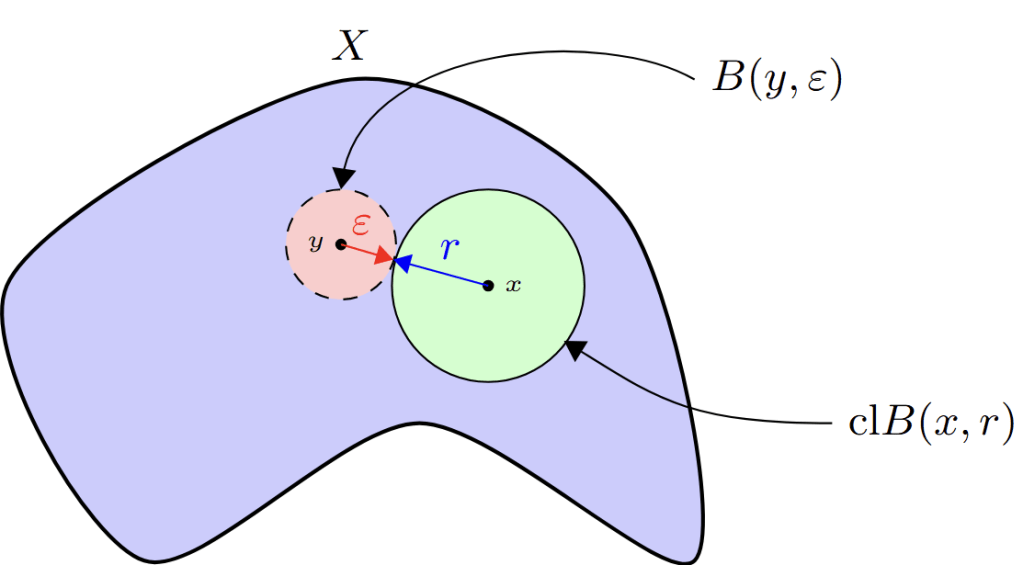
Scratch Work: Consider the metric space $(X,d)$ in blue below. The green disk is the open ball $B(x,r).$ Our goal is to show that $B(x,r)$ is an open set in $(X,d).$ This means that for all $y\in B(x,r)$ we must find some radius $\varepsilon>0$ so that $B(y,\varepsilon)\subset B(x,r).$

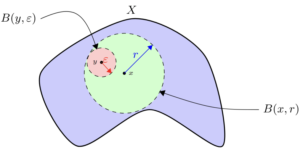
How might we go about this? Well, to show $B(y,\varepsilon)\subset B(x,r),$ we need to show that $z\in B(y,\varepsilon)$ implies $z\in B(x,r).$ That is, $d(y,z)<\varepsilon$ implies that $d(x,z)<r.$ To the rescue, the triangle inequality gives us $d(x,z)\leq d(x,y)+d(y,z) < d(x,y) +\varepsilon .$ But since we want $d(x,y) +\varepsilon <r$ we let $\varepsilon = r- d(x,y) .$ Note that $\varepsilon>0$ since the t$y\in B(x,r).$

Take a moment to work out the geometry here.

Proof: Let $\varepsilon = r- d(x,y) .$ We claim that $B(y,\varepsilon)\subset B(x,r).$ Indeed, let $z\in B(y,\varepsilon)$ and observe that

$$d(x,z)\leq d(x,y)+d(y,z) < d(x,y) +\varepsilon = d(x,y) + r- d(x,y)=r.$$

Thus, $z\in B(x,r).$

Important Remark: Note that $X$ and $\emptyset$ are both open sets in any metric space $(X,d).$ The reason why $X$ is open is that for any $x\in X$ and $r>0$ we have $B(x,r) \subseteq X.$ As for $\emptyset$ being open, note that the statement: for all $x\in \emptyset$ there exists some $r>0$ such that $B(x,r) \subseteq \emptyset$ is true. This is because there are no $x\in \emptyset$ to prove it wrong! Thus, it is vacuously true. Vacuously, in this case, means there are no $x\in \emptyset$ to disprove the statement. Take a moment to appreciate this strangeness!

A challenge left for you is to show that $(a,\infty)$ and $(-\infty,a)$ are open sets in $(\R, d_E).$

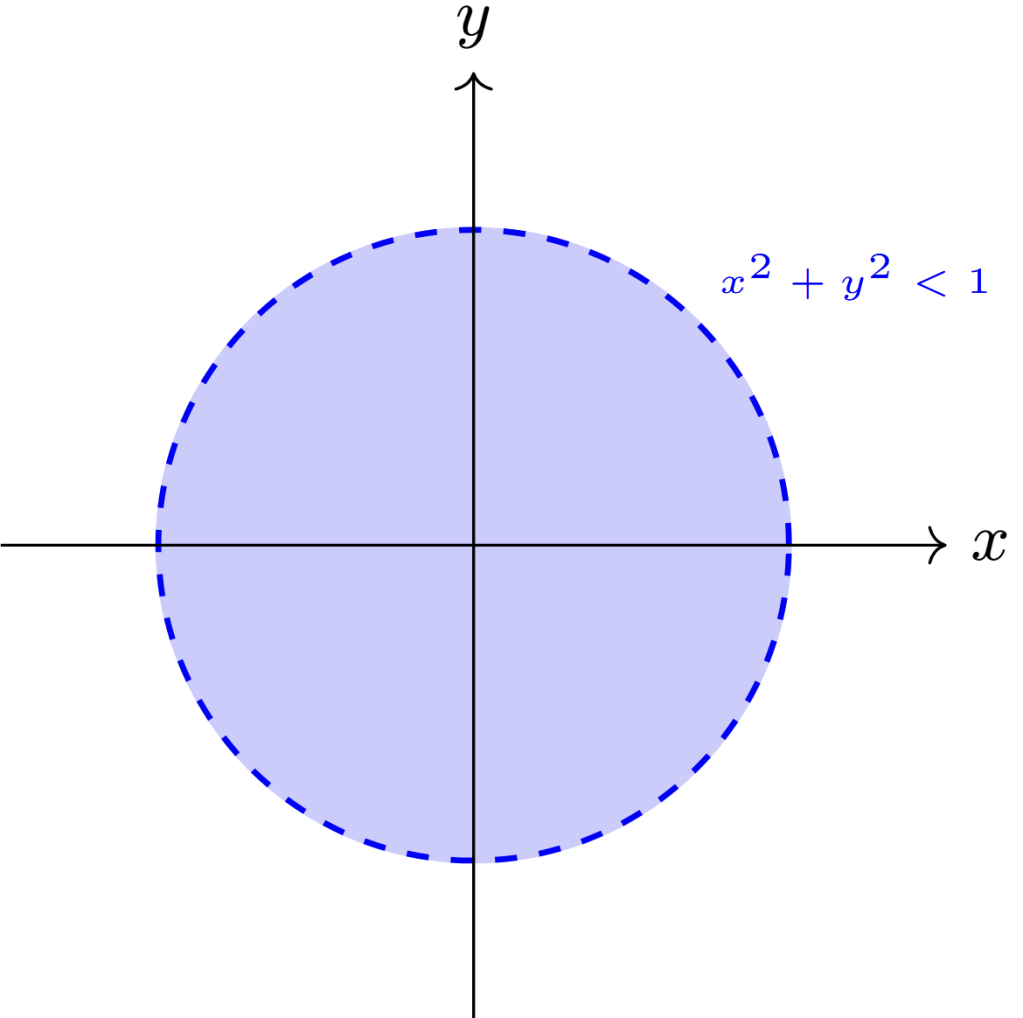
What is $B(\mathbf{0},1)$ in the metric space $(\R^2, d_E)?$

First, note that $B(\mathbf{0},1)$ is the ball centered at the origin of the plane $\mathbf{0} = \langle0,0\rangle\in \R^2$ with radius equal to $1.$ This will be the case for the next few examples.

With the Euclidean metric, we are interested in finding all the points that are within a distance of $1$ of the origin. Give this a go!

Solution: (Click in the Discovery)

As you might have guessed, it’s a circle since $d_E$ is given by the Pythagorean theorem.

What is $B(\mathbf{0},1)$ in the metric space $(\R^2, d_M)?$

Solution: (Click in the Discovery)

Recall that $d_M$ is given by the equation,

$$d_M(x,y) = |x_1-y_1| +|x_2-y_2|.$$

Which for us with $y_1=y_2 = 0$ gives, the equation, using the standard variables, $|x| + |y| < 1.$

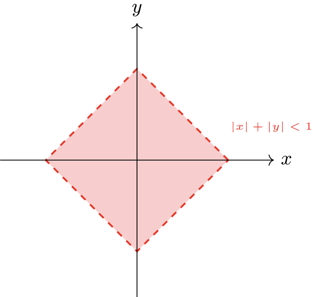
How strange, an open ball is a square!

What is $B(\mathbf{0},1)$ in the metric space $(\R^2, d_{\infty})?$

Solution: (Click in the Discovery)

Since $d_{\infty}$ is given by,

$$d_{\infty}(x,y) = \max{\big\{|x_1-y_1|\,,\,|x_2-y_2|\big\}},$$

We are looking for all the points whose coordinate values, $\langle x,y\rangle ,$ are less than 1 in absolute value.

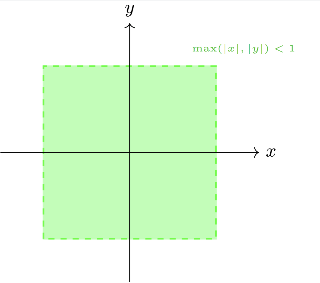
How strange, an open ball is a square! (Again!)

What are some open sets in the metric space $([0,1], d_E)?$

Now that we have seen some open sets and open balls, let’s ask a trickier question. What are some open sets in the metric space $([0,1], d_E)?$This is trickier because we now want an open set $U\subset [0,1].$ And, $[0,1]$ is itself a subset $[0,1]\subset \R.$ We will see why this makes some things seem strange.

First, let me say that we’re abusing notation a little here when we write $( [0,1],d_E).$ So, to avoid needless confusion, the set we are considering is the closed unit interval $[0,1]$ and the metric is the absolute value $d_E(x,y) = |x-y|$ for all $x,y\in [0,1].$

There are some obvious open sets in $([0,1], d_E),$ such as $(0.2\,,\, 0.3)\subset [0,1].$ However, we claim that $[0\,,\, 0.3)\subset [0,1]$ is also an open set in our metric space, even if it doesn’t look like it. See if you can see why!

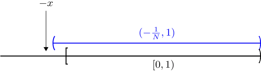
For $[0\,,\, 0.3)\subset [0,1]$ to be an open set, we need to show that every point $x\in [0\,,\, 0.3)$ has an open ball that is centered at $x$ and lies completely inside $[0\,,\, 0.3).$ Of course, the trouble point in the interval is $0\in [0\,,\, 0.3).$ So we focus on 0. Consider the open ball $B(0,\,0.1).$ By definition,

Well, the only points $y\in [0,1]$ with $|y|<0.1$ are those contained in $[0,0.1).$

But this set is contained in the set $[0\,,\, 0.3).$ That is, $[0, 0.1)\subset [0, \,0.3).$

The reason we have square brackets around zero is, first, because $0\in B(0,\,0.1)$ and, second, because there are no other points less than zero in our metric space’s set $X=[0,1].$ Thus, we see that open sets don’t need to look open at first.

See if you can argue why $(0.9\,,\, 1]\subset [0,1]$ and $[0\,,\, 1)\subset [0,1]$ are open sets in $([0,1], d_E)$ as well!

Remark: This is a little taste of what are called subspaces and relative openness. However, we will wait to cover this in more detail in another article.

Closed Sets

We have yet to mention what a closed set is, although we did mention what a closed ball is. So, we might think that we will define a closed set using closed balls. However, this is not the case! We define them in terms of their complement.

Definition (Closed Set): Let $(X,d)$ be a metric space. We call a subset $E\subseteq X$ a closed set in $X$ if its complement $X\setminus E$ is an open set.

Recall that the complement of a set is everything that is not in the set, i.e. $X\setminus E = \{y\in X\;:\;y\notin E\}.$

Remark: Note this shows why $[a,b]\subset \R$ is a closed interval. It’s because $\R\setminus [a,b] = (-\infty,a)\cup (b,\infty)$ is open!

Challenge: Show that closed balls are closed sets.

Proof: (Click in the Discovery)

Scratch: We aim to show that $\mathrm{cl}{B}(x,r) := \{z\in X\;:\;d(x,z)\leq r \}$ is a closed set. We do this by showing that $X\setminus \mathrm{cl}{B}(x,r) = \{z\in Z\;:\;d(x,z)>r\}$ is an open set. Recall, to show that $X\setminus \mathrm{cl}{B}(x,r)$ we must show that for every point $y\in (X\setminus \mathrm{cl}{B}(x,r) )$ there is some $\varepsilon>0$ such that $B(y,\varepsilon)\subset X\setminus \mathrm{cl}{B}(x,r) .$

To show $B(y,\varepsilon)\subset X\setminus \mathrm{cl}{B}(x,r)$ we want to show that $z\in B(y,\varepsilon)$ implies $z\in X\setminus \mathrm{cl}{B}(x,r) .$ That is,

$$d(y,z)r.$$

Well, using the triangle inequality, we want to have $d(x,z)$ greater than something. This means that we want to look at the distance between $x$ and $y,$ or $y$ and $z$ this is because we will have something like $d(\cdot,\cdot)\leq d(x,z) + d(\cdot,\cdot)$ which has $d(x,z)$ on the correct side of the inequality. In particular, we consider

$$d(x,y)\leq d(x,z)+d(y,z) < d(x,z)+\varepsilon$$

Which gives $d(x,z)> d(x,y) -\varepsilon,$ and since we want $d(x,z)> r$ we claim letting $\varepsilon = d(x,y)-r$ works. We leave it to you to write out the formal proof! You’re welcome!

Intersections and Unions of Open and Closed Sets

We have two goals left for this article, and they concern taking the union and intersection of open sets and the union and intersection of closed sets. These might seem like strange things to want to consider; however, when we eventually look at the axioms of a topological space, we will see these results come into play.

Arbitrary Unions/Intersections of Open Sets

The goal is to answer the following questions:

1. Is the arbitrary union of open sets an open set?
2. Is the arbitrary intersection of open sets an open set?

Take a moment to think about these questions and make a guess!

---

The answer to 1 is yes and 2 is no. We will demonstrate these both in a few moments; however, let’s ask something weaker than question 2. Is finite intersections of open sets open? As it turns out, yes, yes they are! Let’s see why.

Theorem (Arbitrary Unions and Finite Intersections of Open Sets): Let $(X,d)$ be a metric space and let $U_{\alpha}\subseteq X$ be an open set in $X$ for all $\alpha \in I$ where $I$ is an arbitrary index set. Then, the following properties hold:

1. The set $\bigcup_{\alpha\in I}U_{\alpha}$ is an open set.
2. If $\{U_1,\cdots,U_N\}$ is a finite collection of open sets, then the intersection $\bigcap_{n=1}^NU_{n}$ is open.

Proof: (Click in the Discovery)

Proof of 1. Here’s the idea. To show that $\bigcup_{\alpha\in I}U_{\alpha}$ is an open set, we must show that every $x\in \bigcup_{\alpha\in I}U_{\alpha}$ has some $r>0$ such that $B(x,r)\subset \bigcup_{\alpha\in I}U_{\alpha}.$ Indeed, this is the case since $x\in \bigcup_{\alpha\in I}U_{\alpha}$ implies that $x\in U_{\alpha_0}$ for some $\alpha_0\in I.$ And, since $U_{\alpha_0}$ is an open set, there is some $r>0$ such that $B(x,r)\subset U_{\alpha_0}\subset \bigcup_{\alpha\in I}U_{\alpha}.$

Proof of 2. Let $x\in \bigcap_{n=1}^NU_{n}.$ We aim to show that there is some $r>0$ such that $B(x,r)\subset \bigcap_{n=1}^NU_{n}.$ Well, $x\in \bigcap_{n=1}^NU_{n}$ implies that $x\in U_{n}$for $1\leq n\leq N.$ Consequently, there are $N$ radii $r_1,\cdots,r_N>0,$such that $B(x,r_n)\subset U_{n}$ for $1\leq n\leq N.$ Let’s simply take the smallest radii $r:=\min\{r_1,\cdots,r_N\},$ which we can guarantee is greater than zero since we are taking a minimum of a finite collection of positive numbers $r_1,\cdots,r_N>0.$ Thus, we have $B(x,r)\subset U_{n}$ for all $n,$ and consequently, $B(x,r)\subset \bigcap_{n=1}^NU_{n}.$

We have a nice corollary!

Corollary (Another Characterization of Open Sets): Let $(X,d)$ be a metric space. We call a subset $U\subseteq X$ an open set in $X$ if and only if $U$ can be written as the union of open balls in $(X,d).$

Proof: (Click in the Discovery)

Forward: Let $U\subseteq X$ be an open set in $X.$ It follows that for all $x\in U$ there is some $r_x>0$ such that

$$B(x,r_x) \subseteq U.$$

Thus,

$$U = \bigcup_{x\in X} B(x,r_x).$$

Note that we are unioning over $x\in X.$

Backward: Let $U$ be a union of open balls in $X.$ By Theorem 1 and the fact that open balls are open sets, $U.$

Now, let’s go back to show that an arbitrary intersection of open sets is not, in general, an open set.

Proposition (Arbitrary Intersections of Open Sets is NOT Open): Consider $(\R,d_E)$ and the collection of open sets (intervals)

$$\mathcal{C} = \left\{\left(-\frac{1}{n}\,,\,1\right) \;:\; n\in \N \right\}.$$

Then, the intersection of all open intervals in $\mathcal{C}$ is not an open set.

Give it a go and see what you get!

Proof: (Click in the Discovery)

First, note that

$$\left(-\frac{1}{n+1}\,,\,1\right) \subsetneq \left(-\frac{1}{n}\,,\,1\right) .$$

Next, we claim that the intersection $\bigcap_{n\in \N}\left(-\frac{1}{n}\,,\,1\right) = [0,1).$ To see this is the case, note that we definitely have $[0,1)\subset \bigcap_{n\in \N}\left(-\frac{1}{n}\,,\,1\right)$ since we have $[0,1)\subset\left(-\frac{1}{n}\,,\,1\right)$ for all $n\in \N.$ We just have to show that no negative numbers are in our intersection.

To see that no negative number is in our intersection, suppose for the hope of a contradiction, that some $-x\in \bigcap_{n\in \N}\left(-\frac{1}{n}\,,\,1\right)$ where $-x<0.$ It follows (by the Archimedean Property in this article) that there is some $N\in \N$ large enough so that $\frac{1}{n}<x.$ Consequently, $-x<-\frac{1}{N}.$ Thus, see that $-x\notin \left(-\frac{1}{N}\,,\,1\right)$ and therefore, $-x\notin \bigcap_{n\in \N}\left(-\frac{1}{n}\,,\,1\right)$ our contradiction.

Thus, no negative number is in our intersection proving our claim that the infinte intersection of open sets can be a non-open set,

$$\bigcap_{n\in \N}\left(-\frac{1}{n}\,,\,1\right) = [0,1).$$

This wasn’t too bad, right? The good news is that we are basically done since closed sets are defined in terms of open sets, we can use Theorem 1 to answer the same questions regarding closed sets.

Arbitrary Unions/Intersections of Closed Sets

Same as before,

1. Is the arbitrary union of closed sets an closed set?
2. Is the arbitrary intersection of closed sets an closed set?

As a hint, if you know De Morgan’s Laws (applied to sets) use them!

---

Ok, the answer here follows from what are known as De Morgan’s Laws.

Theorem (De Morgan’s Laws): Let $\{E_i\}_{i\in I}$ be a collection of subset of the set $X.$ Then we have the following,

$$X \setminus \bigcap_{\alpha \in I} E_{\alpha} = \bigcup_{\alpha\in \mathcal{I}}(X\setminus E_{\alpha}),$$

and

$$X \setminus \bigcup_{\alpha \in I} E_{\alpha} = \bigcap_{\alpha\in \mathcal{I}}(X\setminus E_{\alpha}).$$

Note that the index set $I$ can be finite, countably infinite, uncountably infinite, etc. It’s arbitrary.

Remark: Note that this is a statement about how taking complements interacts with unions and intersections. What’s great is that these laws are statements about sets, so to prove them we don’t need to use anything about openess/closedness.

Proof: (Click in the Discovery)

We will prove the first statement and leave you to prove the other since the proof is similar. That is, we will show the following set relation,

$$X \setminus \bigcap_{\alpha \in I} E_{\alpha} = \bigcup_{\alpha\in \mathcal{I}}(X\setminus E_{\alpha}).$$

To begin, we show $X \setminus \bigcap_{\alpha \in I} E_{\alpha} \subset \bigcup_{\alpha\in \mathcal{I}}(X\setminus E_{\alpha}).$

With this goal in mind, let $x\in X \setminus \bigcap_{\alpha \in I} E_{\alpha} .$ Now observe

$$x\in X \setminus \bigcap_{\alpha \in I} E_{\alpha} \iff x\notin \bigcap_{\alpha\in \mathcal{I}}E_{\alpha} .$$

The right-hand only holds if and only if there is some $\alpha_0\in I$ such that $x\notin E_{\alpha_0},$ which is equivalent to the statement $x\in X\setminus E_{\alpha_0}.$ Which implies

$$x\in \bigcup_{\alpha\in \mathcal{I}}(X\setminus E_{\alpha}).$$

Thus, $X \setminus \bigcap_{\alpha \in I} E_{\alpha} \subset \bigcup_{\alpha\in \mathcal{I}}(X\setminus E_{\alpha})$ as desired.

Now, note that almost all of our steps were bidirectional, that is, if and only if statements. Thus, with minor modifications, we can just use the same logic to prove the other set inclusion $\bigcup_{\alpha\in \mathcal{I}}(X\setminus E_{\alpha})\subset X \setminus \bigcap_{\alpha \in I} E_{\alpha}.$ Thus concluding the proof.

With De Morgan’s Laws by our sides, we can now answer our questions!

Theorem (Finite Unions and Arbitrary Intersections of Closed Sets): Let $(X,d)$ be a metric space and let $E_{\alpha}\subseteq X$ be a closed set in $X$ for all $\alpha \in I$ where $I$ is an arbitrary index set. Then, we have the following properties hold:

1. If $\{E_1,\cdots,E_N\}$ is a finite collection of closed sets, then the union $\bigcup_{n=1}^N E_{\alpha}$ is a closed set.
2. The arbitrary intersection $\bigcap_{n=1}^N E_{n}$ is closed.

Proof: (Click in the Discovery)

Proof of 1. Let $\{E_1,\cdots,E_N\}$ is a finite collection of closed sets. We want to show that

$$\bigcup_{n=1}^N E_{\alpha}$$

is closed. We do so by demonstrating that $X\setminus \bigcup_{n=1}^N E_{\alpha}$ is open. See where we will use De Morgan’s Laws?

Since $\{E_1,\cdots,E_N\}$ is a finite collection of closed sets, $\{X\setminus E_1,\cdots, X\setminus E_N\}$ is a finite collection of open sets, and therefore their intersection is open. That is$\bigcap_{n=1}^N(X\setminus E_{n})$ is open. But by De Morgan’s Laws,

$$X \setminus \bigcup_{n=1}^N E_{n} = \bigcap_{n=1}^N(X\setminus E_{n}).$$

So that $X\setminus \bigcup_{n=1}^N E_{\alpha}$ is open. Hence $\bigcup_{n=1}^N E_{\alpha}$ is closed, as desired.

Thus, $X\setminus \bigcup_{n=1}^N E_{\alpha}$ and

Proof of 2. In a similar manner as before, we want to show that

$$\bigcap_{\alpha \in I} E_{\alpha}$$

is closed. We do so by showing that $X\setminus \bigcap_{\alpha\in I} E_{\alpha}$ is open.

Since $\{E_{\alpha}\}_{\alpha\in I}$ are closed, $\{X\setminus E_{\alpha}\}_{\alpha\in I}$ are open. Thus, their union is open: $\bigcup_{\alpha\in I}(X\setminus E_{\alpha}) = \mathrm{open.}$ By De Morgan’s Law,

$$X \setminus \bigcap_{\alpha \in I} E_{\alpha} = \bigcup_{\alpha\in \mathcal{I}}(X\setminus E_{\alpha}),$$

and $X\setminus \bigcap_{\alpha\in I} E_{\alpha}$ is open. As desired.

Final Remarks

We have covered a lot of stuff today. I hope that you found it helpful, if not, please leave a comment indicating where I could have done better. Thank you in advance!

There is a lot more we could have covered about metric spaces than we did today. We didn’t even touch sequences or continuity yet! We will cover these in the future! However, in the meantime, there are some great resources out there for you in your mathematical journey. I will list a few of my favorites for you to peruse,

• Introduction to Metric Spaces | Mathematics | MIT OpenCourseWare This is a free MIT course with lecture videos, lecture notes, and problem sets.
• Introduction to Topology: Second Edition (Dover Books on Mathematics): Gamelin, Theodore W., Greene, Robert Everist. This is an Amazon link (with no royalties) for convenience.
• Amazon.com: Principles of Mathematical Analysis (International Series in Pure and Applied Mathematics): Rudin, Walter: Books This is another Amazon link (with no royalties) for convenience.
• Metric Space | Brilliant Math & Science Wiki Less comprehensive than the other sources, but it’s free and covers continuity. I will say that I haven;t looked at this article, but Brilliant usually does a great job.

Be Kind. Be Curious. Be Compassionate. Be Creative.

And Have Fun!

---

Footnote(s):

1. This happens all the time in math, for instance, to form a group, $(G,\star),$ we have a set $G$ with an operation $\star$ on the set that satisfies certain axioms. ↩︎
2. The supremum of a set of real numbers equals the least upper bound of that set. For example, the set $[0,2]$ has $\sup{\{[0,2]\}}=2.$ Similarly, $\sup{\{(0,2)\}}=2.$ This is because $2$ is an upper bound for $(0,2)$ and there is nothing smaller that is an upper bound. One way of thinking of the supremum is to think of it as quantifying what the maximum of the set wants to be. For instance, clearly the maximum element in $[0,2]$ is $2.$ And, for the open interval $(0,2)$ the number $2$ really wants to be the upper bound, but since $2\notin (0,2)$ it cannot be the maximum. However, it can be the supremum! In fact, the supremum equals the maximum if it belongs to the set in question. For more detail, see this article here. Or, just change $\sup{}$ with $\max{}$ everywhere and it all works out. ↩︎
3. To see why, we employ some calculus. Consider $\sin{(2\pi x)}-\cos{(2\pi x)}.$ To find its maximum (or minimum), we take its derivative and set it to zero:
   $$\frac{d}{dx}\left( \sin{(2\pi x)}-\cos{(2\pi x)} \right) = 2\pi\left(\cos{( 2\pi x)}+\sin{(2\pi x)}\right)=0.$$Which is solved by $x_0 = 3/8 \in [0,1].$ Now, plugging this into $|\sin{(2\pi x)}-\cos{(2\pi x)}|$ we get $\sqrt{2}.$ ↩︎