Permutation Groups

I’ve recently started a new research project that has connections to permutation groups. For this reason, I thought that I would write an article about them so that friends and family could learn a little math regarding what I might be thinking about for the next few months! But you don’t care about that! You just want/need to learn about permutation groups, I mean… you clicked on the link! So, let’s just get into this!

What’s A Permutation?

Loosely speaking, a permutation is a rearrangement of the order of objects (we will focus on a finite list of objects). It doesn’t matter what objects we want to rearrange the order of. For example, when we shuffle playing cards, we are permuting their order. Or, when we make anagrams of a bunch of letters, we are finding permutations of the list of letters. But, since we all love math(s) and numbers, we will focus on permuting (rearranging) the numbers $1,2,3,4,\cdots ,n$ when we want to consider a permutation of $n$ objects. This makes it easier to type and do out examples since we are focusing on a concrete list of objects, e.g., numbers! From now on, we’ll denote the set of positive integers up to and including $n$ by $[n]$ .

$[n]:=\{ 1,2,3,\cdots, n\}.$

Consider the special case of $n=3$ . We want to count how many different ways we can rearrange the numbers $[3]:=\{ 1,2,3\}$ there are. I.e. how many permutations are there of the numbers 1, 2, and 3?

Answer: There are $3! = 3\cdot2\cdot1 = 6$ permutations. To see why, observe that we have 3 options for what number to put first. Once we fix the first number, we have two numbers left to choose from for the second number. Lastly, after we fixed the first two numbers, we have only one number left, so 1 option for the third number. Altogether, we have $3! = 3\cdot2\cdot1 = 6$ ways to order the numbers 1, 2, and 3. (For a more detailed explanation of general counting problems, consider checking out Math That Counts.)

What we want to do is consider the act of permuting the numbers 1, 2, 3. For example, let $\epsilon$ be a fancy way of denoting: do nothing. So that, if we started with the order 1, 2, 3 and then applied $\epsilon$ would give 1, 2, 3 again. Likewise, applying $\epsilon$ to 3, 1, 2 would give 3, 1, 2 again.

$1, 2, 3, \overset{\epsilon}{\longmapsto} 1, 2, 3 \qquad \qquad 3, 1, 2\overset{\epsilon}{\longmapsto} 3, 1, 2$

Or, let $\alpha$ denote: swap the 1 and 2. Then, starting with 1, 2, 3 and applying $\alpha$ would give, 2, 1, 3. Or, applying $\alpha$ to 2, 3, 1, would give 1, 3, 2.

$1, 2, 3, \overset{\alpha}{\longmapsto} 2, 1, 3 \qquad \qquad 2, 3, 1, \overset{\alpha}{\longmapsto} 1, 3, 2$

Yet another example could be letting $\beta$ denote: swap 1 with 3 and then swap 2 with 1. A mouthful, but would cause 1, 2, 3, to become 3, 1, 2. Or it would permute 2, 1, 3 to become 1, 3, 2.

$1, 2, 3, \overset{\beta}{\longmapsto} 3, 1, 2 \qquad \qquad 2, 3, 1, \overset{\beta}{\longmapsto} 1, 3, 2$

But why stop with only $\alpha$ and $\beta$ ? Why not apply $\alpha$ and then $\beta$ ??? Well, this would mean: swap the 1 and 2 and then swap 1 with 3 and then swap 2 with 1. Starting with 1, 2, 3 we’d end up with:

$1, 2, 3, \overset{\alpha}{\longmapsto} 2, 1, 3 \overset{\beta}{\longmapsto} 1, 3, 2.$

So, we can combine these actions in some way. Let’s try and apply $\alpha$ and then $\alpha$ again! This would mean: swap the 1 and 2 and then swap the 1 and 2 (again). This would result in:

$1, 2, 3, \overset{\alpha}{\longmapsto} 2, 1, 3 \overset{\alpha}{\longmapsto} 1,2,3.$

But, this is the same as applying $\epsilon$ to 1,2,3. So, in some sense $\epsilon = \alpha\alpha$ .

These operations, these permutations and combinations thereof ( $\epsilon, \alpha, \beta, \beta\alpha, \alpha\beta, \alpha\alpha$ ) are what we are interested in studying.

Let’s Make This More Mathy

It’s now time to develop the mathematical machinery. Let’s begin by defining mathematically what we mean by a permutation:

Definition (Permutation): Let $S$ be a set and let $f$ be a function $f:S \rightarrow S$ . If the $f$ is both injective and surjective (by definition, $f$ is bijective)¹ we call $f$ a permutation of $S$ . Or, if there is a one-to-one correspondence between $x\in S$ and $f(y)\in S$ then we call $f$ a permutation of $S$ .

Great! Therefore, when we want to study permutations, we really are studying bijective functions. But, if all this terminology like injective, surjective, bijective is too abstract for you, then use the loose definition we said earlier: a permutation is a rearrangement of the order of objects. You won’t miss out on anything in this article using the loose definintion.

We are going to study the set of all permutations of $[n]$ . Let’s denote the set $S_n$ as the set of permutations of the numbers in $[n]$ ,

$S_n :=\;\textit{ }\;$ $\textit{ }\;\;\{$ the set of all permutations of $[n]$ $\}$

For example, we know that $\alpha \in S_3$ from earlier. Likewise, $\epsilon \in S_3$ and $\beta \in S_3$ . We also know that $\alpha\beta \in S_3$ , which can be thought of a function composition of $\alpha$ and $\beta$ . We will call this multiplying the permutations $\alpha$ and $\beta$ . This means that there is more to $S_n$ and just its elements; there is structure to how we can combine the elements in $S_n$ . It turns out $S_n$ is what we call a group.

Note, when we write $\beta \alpha$ we are going to read the composition from right to left. This is the same way you’d read $(g\circ f )(x)$ . Which means apply $f$ to $x$ first and then apply $g$ to what results from $f(x)$ to get $g(f (x))$ .

It’s a Group!

Recall the definition of a group (and for those who have not seen group theory, don’t worry! We will explain each step)

Definition (Group): Let $G$ be a set and $*$ denote a binary operation². Then, we call $(G,*)$ a group if the following are true:

The operation is associative, i.e. $g*(h*k) = (g*h)*k$ for all $g,h,k \in G$ ,
there is an identity element $\epsilon \in G$ where $g* \epsilon = \epsilon* g= g$ for all $g \in G$ , and
for all $g \in G$ there exists an inverse $g^{-1} \in G$ such that $g*g^{-1} = g^{-1}*g = \epsilon$ .

When the operation is known, we will write that $G$ is a group and drop the operation symbol from (G,*). Similarly, we will write $ab$ instead of $a*b.$

We claim that $S_n$ along with function composition forms a group.

Theorem (The Permutation Group): The set $S_n$ along with function composition forms a group. Moreover, $|S_n| = n!$ .

We aren’t going to go through a fully rigorous proof of this fact, but we will explain the thoughts behind each point.

1) Associativity

Since, by definition, a permutation is a bijective function we can use that function compositions are associative to say,

for all $\alpha,\beta,\gamma \in S_n$ we have $(\alpha \beta) \gamma = \alpha (\beta \gamma)$ .

*Note, it would be more accurate to write $\alpha \circ \beta$ and not $\alpha \beta$ for their combination.³

2) Identity

Recall, $\epsilon \in S_3$ meant to do nothing. We can define a similar element for any $S_n$ . We call $\epsilon$ our identity element because it preserves the identity of the numbers $1, 2, 3, \cdots , n.$

*Note, $\epsilon$ is the function such that $\epsilon(m) = m$ for all $m\in [n]$ .

3) Inverses

Since we are permuting our numbers 1 through n, we could always undo what we did to get back to how we started. For instance, $\alpha$ meant: swap the first two numbers in $S_3$ . If we applied $\alpha$ again then we would have swapped the first two back again, or $\alpha \alpha = \epsilon.$ In a similar way, $\beta$ wanted us to shift each of the numbers one location. We can undo that with another permutation, call it $\delta$ . Then, we’d have

$\beta \delta = \delta \beta = \epsilon$ .

This is true in general, for any $\sigma \in S_n$ there is an inverse element denoted $\sigma^{-1}$ such that $\sigma\sigma^{-1} = \sigma^{-1} \sigma = \epsilon$ .

*Note, we can do this because bijective functions have inverses.

“ $\square"$

Since $S_n$ forms a group with the operation of function composition, we can use tools from group theory to start analyzing our permutations! Woot woot! But before we do, let’s find a convenient way to express some permutations $\alpha \in S_n$ other than using sentences like: swap blah and blah with blah and blah…

Two-Line Notation

It’s NOT a Matrix

The easiest way to express some permutation $\alpha \in S_n$ is using the two-line notation. It may look like a matrix, however, it’s not! You don’t perform matrix multiplication when you combine two permutations!

Let’s begin with the identity we saw already $\epsilon \in S_3.$ Recall that the identity permutation denotes: do nothing. To express this idea, we will begin by writing our elements in $[n]$ on the top row:

$\epsilon = \begin{pmatrix} 1 & 2 & 3\\ & & \end{pmatrix}.$

Under each of the numbers 1, 2, and 3 we write where $\epsilon$ sends them. Since every number is `sent to itself’

$\epsilon = \begin{pmatrix} 1 & 2 & 3\\ 1& 2 & 3 \end{pmatrix}.$

Let’s take another example. Recall $\alpha \in S_3$ . Begin by writing 1, 2, 3, in the top row:

$\alpha = \begin{pmatrix} 1 & 2 & 3\\ & & \end{pmatrix}$

We had $\alpha$ denote: swap the 1 and 2. So that,

$\alpha = \begin{pmatrix} 1 & 2 & 3\\ 2 & 1 & \end{pmatrix}$

Last, but not least, $\alpha$ sends 3 to 3. Thus, we have

$\alpha = \begin{pmatrix} 1 & 2 & 3\\ 2 & 1 & 3 \end{pmatrix}.$

One more bit of notation. Since $\alpha$ sends 1 to 2 we can denote this by writing $\alpha(1) = 2$ or by $1 \overset{\alpha}{\longmapsto} 2$ . And, if we were to apply $\alpha$ more than once, we would write $\alpha^m(1)$ instead of $\alpha(\alpha(\cdots \alpha(1)\cdots))$ for example, $\alpha^2(1) = \alpha(\alpha(1))$ .

Let’s do one more example! Recall the permutation $\beta\in S_3$ from before. Again, begin by writing out the first row,

$\beta= \begin{pmatrix} 1 & 2 & 3\\ & & \end{pmatrix}$

Using that $\beta$ denotes: swap 1 with 3 and then swap 2 with 1, we place a 3 under the 1 and a 1 under the 3,

$\beta= \begin{pmatrix} 1 & 2 & 3\\ 3 & & 1 \end{pmatrix}$

Next, we must swap 2 and 1. Thus, in the bottom row, we swap the 1 under the 3 with a 2, and the 1 goes under the 2:

$\beta= \begin{pmatrix} 1 & 2 & 3\\ 3 & 1 & 2 \end{pmatrix}.$

Not so bad.

If we know where some number $n$ goes after the permutation, then we can write the two-line notation for the permutation. In all its glory, we write:

$\alpha= \begin{pmatrix} 1 & 2 & 3 & \cdots & n\\\alpha(1) & \alpha(2) & \alpha(3) & \cdots & \alpha(n)\end{pmatrix}.$

for $\alpha \in S_n.$

How do you Multiply Permutations?

Now that we have a way to write $\alpha$ and $\beta$ , how would we write $\beta \alpha$ given the two-line notation from earlier? Well, we DO NOT MULTIPLY the two-line notations like matrixes. This is not an issue for our examples since we cannot multiply a 3×2 matrix with a 3×2 matrix.

What we DO do⁴ is simply ask, where would # end up after we apply $\alpha$ and then $\beta$ ? Continuing with

$\alpha = \begin{pmatrix} 1 & 2 & 3\\ 2 & 1 & 3 \end{pmatrix}$ and $\beta= \begin{pmatrix} 1 & 2 & 3\\ 3 & 1 & 2 \end{pmatrix}.$

Note that $\alpha$ sends 1 to 2. Then, $\beta$ sends 2 to 1. Thus, $\beta (\alpha ( 1) ) = \beta (2) = 1$ ,

$\beta \alpha= \begin{pmatrix} 1 & 2 & 3\\ 1 & & \end{pmatrix}$

Now, let’s ask where 2 goes. Well, $\alpha$ sends 2 to 1. Then, $\beta$ sends 1 to 3. Thus, $\beta (\alpha ( 2) ) = \beta (1) = 3$ ,

$\beta \alpha = \begin{pmatrix} 1 & 2 & 3\\ 1 & 3 & \end{pmatrix}$

Lastly, $\alpha$ sends 3 to 3. Then, $\beta$ sends 3 to 2. Thus, $\beta (\alpha ( 3) ) = \beta (3) = 2$ ,

$\beta \alpha = \begin{pmatrix} 1 & 2 & 3\\ 1 & 3 & 2 \end{pmatrix}$

Again, not so bad. Well, not so bad once you get used to it!

Cycle Notation

Mathematicians are ~~lazy~~ efficient people, and they invented an even better method to write down permutations that requires less writing! It has only one line!

What is it?

I will admit, cycle notation can be tricky to get used to, but once you do it will be your best friend when working with permutations. We’ll show how it works through an example. Let’s take the large permutation:

$\sigma = \begin{pmatrix} 1 & 2 & 3 &4 &5 & 6\\ 2 & 1 & 4 & 5 & 3 & 6\end{pmatrix} \in S_6$ .

Take a moment to understand what this permutation is telling us. Once you feel ready, keep reading.

We are going to set up the cycle notation for $\sigma$ in the following way: Start with the number 1.

$\sigma = (1, \qquad )$

and ask, where does $\sigma$ send 1? I.e. $\sigma(1) = ???$ In our situation, $\sigma(1) = 2$ . So, we write 2 next to the 1.

$\sigma = (1 ,2,\qquad )$

Now, ask where does $\sigma$ send 2? Answer: $\sigma(2) = 1$ . Since we are back to where we started (i.e. 1) we close the set of parentheses,

$\sigma = (1 ,2)\cdots$

and then open a new set with the smallest number that we have not used yet. In this case, it’s 3

$\sigma = (1 ,2) (3 ,\qquad )$

Where does $\sigma$ send 3? You can go check, but it’s to 4:

$\sigma = (1 ,2) (3 ,4\qquad )$

Where does $\sigma$ send 4? To 5 of course!

$\sigma = (1 ,2) (3 ,4,5\qquad )$

Where does $\sigma$ send 5? Back to 3, and since we are back where we started this set of parenthesis, we close the parenthesis.

$\sigma = (1 ,2) (3 ,4,5)\cdots$

What’s the smallest number not used yet? It’s 6.

$\sigma = (1 ,2) (3 ,4,5)(6,\qquad)$

Since it goes to itself we are done!

$\sigma = \begin{pmatrix} 1 & 2 & 3 &4 &5 & 6\\ 2 & 1 & 4 & 5 & 3 & 6\end{pmatrix} = (1,2)(3,4,5)(6)$ .

When we read a permutation in cycle notation, we read $(1,2)$ as saying 1 goes to 2 and 2 goes to 1. Similarly, $(3,4,5)$ says, 3 goes to 4, then 4 goes to 5, and finally 5 goes back to 3. This is more efficient and can tell us more; there are little loops that form with this permutation. How cool is that!

Let’s convert $\alpha$ into cycle notation. Recall,

$\alpha = \begin{pmatrix} 1 & 2 & 3\\ 2 & 1 & 3 \end{pmatrix}.$

So, we have 1 going to 2, and 2 going to 1. So, we still have $(1,2)$ . The difference is now that 3 stays at 3. Thus,

$\alpha = \begin{pmatrix} 1 & 2 & 3\\ 2 & 1 & 3 \end{pmatrix} =(1,2)(3).$

But, again, mathematicians are efficient so when we have a situation when some number does not swap with anything, such as $\alpha$ and the number 3, we don’t tend to write $(3)$ in the cycle notation of $\alpha$ therefore,

$\alpha = \begin{pmatrix} 1 & 2 & 3\\ 2 & 1 & 3 \end{pmatrix} =(1,2).$

One last thing:

Definition: (Cycle) We call a permutation a cycle $\sigma \in S_n$ if it can be written in the following way: $\sigma = (a_1, a_2,\cdots, a_k)$ where $a_i \neq a_j$ for $i \neq j$ . We’d say that $\sigma$ has length $k$ or is a k-cycle.

Definition: (Disjoint Cycles) Let $\sigma \in S_n$ and $\pi \in S_n$ be two cycles such that,

$\sigma = (a_1, a_2,\cdots, a_k)$ and $\pi = (b_1, b_2,\cdots, b_t)$

Then we call $\sigma$ and $\pi$ disjoint if $a_i \neq b_j$ for all $i$ and $k$ .

With these two bits of terminology we’d say that $\alpha = (1,2)$ is a 2-cycle and $\sigma = (1,2)(3,4,5)(6)$ is not a cycle; however it is made up of a 2-cycle and 3-cycle that are disjoint.

How do we combine permutations in Cycle notation?

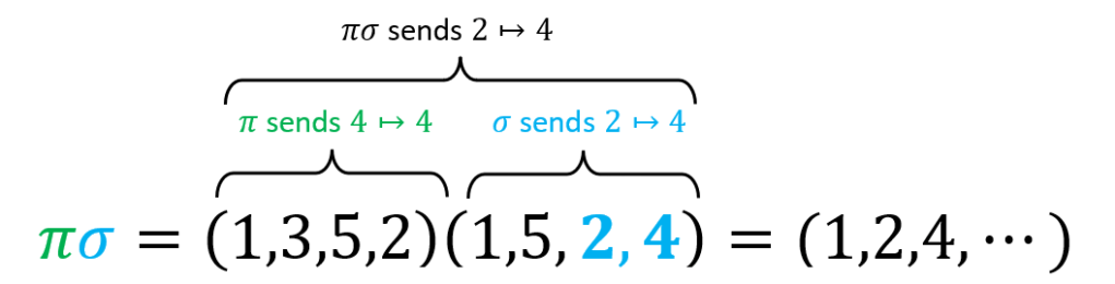
When combining permutations in cycle notation, we basically do the same thing we did earlier. Let’s compute the product of the following permutations:

$\sigma = (1,5,2,4)$ and $\pi = (1,3,5,2)$ .

Where $\sigma, \pi \in S_5.$ We need to remember that we read the product left to right!

Step 1: We begin by determining where 1 will be sent by reading $\pi\sigma = (1,3,5,2)(1,5,2,4)$ right to left. We see that $\sigma$ will send 1 to 5. Next, we now find where $\pi$ sends 5. In this case, to 2. Thus, $\pi\sigma$ sends 1 to 2.

Step 2: Begin with 2 now, since in step 1 we found $1\mapsto 2$ . We find where $\sigma$ sends 2. It turns out $\sigma$ send 2 to 4. Next, we find that $\pi$ does not have a 4 in its cycle. This means that 4 stays at 4. Thus, $\pi\sigma$ sends 2 to 4. See the figure below.

Step 3: Continue but now start at 4. See the figure for all the steps!

Step 1
Step 2
Step 3
Step 4
Step 5

Transpositions

One interesting property that permutation groups enjoy is that any permutation can be written as a product of 2-cycles. In group theory vernacular, $S_n$ is generated by cycles of length two. For this reason, we give 2-cycles a special name:

Definition (Transposition): If $\sigma \in S_n$ is a cycle of length 2 e.g. $(a,b) \in S_n$ where $a,b \in [n]$ and $a\neq b$ , then we call $\sigma$ a transposition.

What we said preceding this definition is captured in the following theorem:

Theorem: Every permutation in $S_n$ can be written as a product of (not necessarily disjoint) transpositions. Although this product is not unique.

Proof: Let $\sigma \in S_n$ be a cycle $\sigma = (a_1, a_2, a_3\cdots, a_k)$ where $a_i \neq a_j$ for $i \neq j$ . Then, we can express $\sigma$ as the following product,

$\sigma = (a_1,a_2)(a_2,a_3)(a_3,a_4)\cdots (a_{k-1},a_k)$ .

To check that the above product is indeed the same as the cycle $\sigma = (a_1, a_2, a_3\cdots, a_k)$ observe that: $a_1$ is not in any of the first $k-2$ transpositions and the $k-1^{st}$ transposition $(a_1,a_2)$ sends $a_1 \mapsto a_2$ just like the $(a_1, a_2, a_3\cdots, a_k)$ does. You can continue with this logic to see that the product is the same as the cycle.

Lastly, we note that any permutation can be written as a product of cycles⁵ and since we can write those cycles as a product of transpositions, we can therefore write any permutation as a product of transpositions.

To see that this product is not unique, consider the products below,

$\sigma = (a_k,a_{k-1})(a_{k},a_{k-2}) (a_k,a_{k-3})\cdots (a_k,a_2) (a_{k},a_1) \\ \textit{ }\;= (a_1,a_k)(a_1,a_{k-1})(a_1,a_{k-2})\cdots (a_1,a_2)$ .

As you can verify (you’re welcome), these are other ways to express $\sigma$ as a product of transpositions.

$\square$

How cool is that! Answer: Very cool!

Even/Odd Permutations

Another reason why we care about transpositions is because we can classify different permutations in terms of how many transpositions they can be written as a product of. For example,

$\delta = (1,2,3,4,5,6) = (1,2)(2,3)(3,4)(4,5)(5,6)$

is made up of 5 transpositions, or simply an odd number of transpositions. Or,

$\lambda = (1,2,3,4,5) = (1,2)(2,3)(3,4)(4,5)$

is made up of 4 transpositions, or simply an even number of transpositions. Or,

$\sigma = (1,5,2,4) = (1,5)(5,2)(2,4)$

is made up of 3 transpositions, or simply an odd number of transpositions.

Wouldn’t it be nice if we could take some permutation group $S_n$ and split it up into two sets of permutations that are either a product of even number or an odd number of transpositions? But we already know that this product is not unique so we cannot… or can we????

It turns out we can! We’ll soon see that no matter how you express, say $\delta$ , as a product of transpositions, $\delta$ , will always need an odd number of them:

$\delta = (1,2,3,4,5,6) = (1,2)(2,3)(3,4)(4,5)(5,6) \\ \textit{ }\qquad\qquad\;\;\;\;\,\,\qquad=(6,5)(6,4)(6,3)(6,2)(6,1)\\ \textit{ }\qquad\qquad\;\;\;\;\,\,\qquad= (1,6)(1,5)(1,4)(1,3)(1,2)(2,3)(4,5)(2,3)(4,5)$

Note these products are made up of 5, 5, and 9 transpositions, which are all odd numbers.

Definition (Even/Odd Permutation): Let $\sigma \in S_n$ be a permutation. We call $\sigma$ an even permutation if we can write $\sigma$ as a product of an even number of transpositions. Likewise, we call $\sigma$ an odd permutation if we can write $\sigma$ as a product of an odd number of transpositions.

Theorem (Even/Odd Permutation Classification): Let $\sigma \in S_n$ be a permutation. Then, $\sigma$ is either an even permutation or an odd permutation, but not both.

Scratch Work: How should be prove that every permutation is either an even or odd permutation, but not both. Well, we already know the first part: every permutation is either even or odd. This is by the previous theorem. The second part: but not both is where the trickiness lies.

The most obvious line of attack is to assume that some permutation can be both even and odd and try to find a contradiction somewhere. So, let $\sigma \in S_n$ be some permutation that is both even and odd. This means that there is a way to write $\sigma$ as a product of an even number of transpositions and a product of an odd number of transpositions. Let’s use $\tau_i$ and $\mu_i$ to denote transpositions. Thus,

$\sigma = \tau_1 \tau_2 \tau_3 \cdots \tau_k = \mu_1\mu_2\cdots \mu_s$ ,

where $k$ is an even number and $s$ is odd. There isn’t much to do other than play around with the above products. Observe that every transposition has the property $(a,b) (a,b) = \epsilon$ so that we can likewise say, $\tau_i \tau_i = \mu_j \mu_j=\epsilon$ . We can use this property when multiplying $\sigma$ on the right by $\mu_s \mu_{s-1}\cdots \mu_2 \mu_1$ to get,

$\tau_1 \tau_2 \tau_3 \cdots \tau_k \mu_{s}\mu_{s-1}\mu_{s-2} \cdots \mu_1= \mu_1\mu_2\mu_3 \cdots \mu_{s-1}\mu_s \mu_s\mu_{s-1}\cdots \mu_3\mu_2\mu_1 \\ \textit{ }\qquad\qquad\qquad\qquad\qquad\;\;\;\;\;\;\,= \epsilon$ .

So we have found a way to express $\epsilon$ as a product of an odd number of transpositions, i.e. $k + s$ transpositions, since we assumed $k$ was even and $s$ was odd. But wait, we also know that $\epsilon = (a,b)(a,b)$ which should make $\epsilon$ an even permutation. Maybe this is the contradiction. If $\epsilon$ is an even transposition, then we have a contradiction since we have found a way to express $\epsilon$ as an odd number ( $k+s$ ) of tranpositions. As it turns out, $\epsilon$ is an even permutation. We will show this in the following lemma:

Lemma (The identity is an EVEN permutation): Let $\epsilon \in S_n$ denote the identity permutation. Then, $\epsilon$ is an even permutation.

Proof of Lemma: Let $\epsilon \in S_n$ denote the identity permutation. We will show that $\epsilon$ is an even permutation using induction. Let $\epsilon = \alpha_1\alpha_2\cdots \alpha_r$ where $\alpha_i$ are transpositions. We will use induction on $r$ .

First note that if $r=1$ , then we’d have $\epsilon = (a_1,a_2)$ . This cannot happen because the identity is not supposed to swap any numbers, yet we’d have $a_1\mapsto a_2$ and $a_2 \mapsto a_1$ . Thus, we’ll prove $r\geq 2$ is even.

Consider when $r=2$ . This is simply the statement we made earlier: $(a_1,a_2) (a_1,a_2) = \epsilon$ .

Now suppose that $\epsilon = \alpha_1\alpha_2\cdots \alpha_r$ for $r>2$ . What we will do is focus on some number in the r^th transposition, $\alpha_r$ , and try to move it to the r-1^st transposition without changing the product. Once we do, we will see that this will then result in two situations: (1) we get a product of two identical transpositions which results in the identity or (2) an eventual contradiction.

Consider the last two transpositions in the product for $\epsilon,\;\alpha_{r-1}\alpha_r$ . We must have one of the following four situations (where $a_1,a_2,a_3,a_4 \in [n]$ and are different):

$\alpha_{r-1}\alpha_r = (a_1,a_2)(a_1,a_2) = \epsilon$

$\alpha_{r-1}\alpha_r = (a_2,a_3)(a_1,a_2) = (a_1,a_3)(a_2,a_3)$

$\alpha_{r-1}\alpha_r = (a_3,a_4)(a_1,a_2) = (a_1,a_2)(a_3,a_4)$

$\alpha_{r-1}\alpha_r = (a_1,a_3)(a_1,a_2) =(a_1,a_2)(a_2,a_3)$

Which you can check by multiplying out the transpositions. When the first situation happens, we then have the product $\epsilon = \alpha_1\alpha_2\cdots \alpha_{r-2}\epsilon = \alpha_1\alpha_2\cdots \alpha_{r-2}$ . But then we have a product of $r-2$ transpositions, which is even by induction. Hence $r$ is even too.

In the second, third, and fourth situations we have moved $a_1$ one transposition to the left. This means that we have one of the following,

$\epsilon = \alpha_1\alpha_2\cdots \alpha_{r-2} (a_1,a_3)(a_2,a_3)$

$\epsilon = \alpha_1\alpha_2\cdots \alpha_{r-2}(a_1,a_2)(a_3,a_4)$

$\epsilon = \alpha_1\alpha_2\cdots \alpha_{r-2} (a_1,a_2)(a_2,a_3)$

Now we play the same game, focus on the transpositions $\alpha_{r-2}(a_1,b)$ where $b = a_2,a_3,a_4$ depending on which situation we have above. We can then remove $a_1$ from the right transposition and put it into the left transposition. This will result in the same four cases as before.

$\alpha_{r-1}(a_1,b)= (a_1,b)(a_1,b) = \epsilon$

$\alpha_{r-2}(a_1,b) = (b,c)(a_1,b) = (a_1,c)(b,c)$

$\alpha_{r-2}(a_1,b) = (c,d)(a_1,b) = (a_1,b)(c,d)$

$\alpha_{r-2}(a_1,b) = (a_1,c)(a_1,b) =(a_1,b)(b,c)$

Where $a_1,b,c,d \in [n]$ and are different. And, just like before, we either have $\alpha_{r-2}(a_1,b) = \epsilon$ , in which case we have found a way to express $\epsilon$ as $r-2$ transpositions, which is even by induction. Hence $r$ is even too. Or, we have one of the bottom three cases in which case we play the same game again on the final three cases.

This process must come to an end either by resulting in case 1, or by moving $a_1$ all the way to the beginning of the product. We claim, however, the latter cannot happen.

Consider what would happen if we were able to remove $a_1$ from all the transpositions in the product, except for the first transposition. This would mean that:

$\epsilon = (a_1, b_1)(b_2,b_3)\cdots(b_{2r-2},b_{2r-1})$

where $a_1\neq b_i$ for all $i$ . We have found a contradiction; we have just concluded that $\epsilon(a_1) = b_1$ . Which cannot be the case since $\epsilon$ is the identity. Therefore, when we are moving $a_1$ we must get a product of identical transpositions to cancel like in case 1. When this happens, we’ve found a product for $\epsilon$ made of $r-2$ transpositions, which is even by induction and thus $r$ is even.

$\square$

Proof of Theorem (Even/Odd Permutation Classification): Assume for the hope of a contradiction that $\sigma \in S_n$ could be written as a product of an even number of transpositions and an odd number of transpositions:

$\sigma = \tau_1 \tau_2 \tau_3 \cdots \tau_k = \mu_1\mu_2\mu_3 \cdots \mu_s$

where $\tau_i$ and $\mu_i$ are transpositions and $k$ is an even number and $s$ is odd. Observe that, for any transposition $(a_1,a_2)$ we have $(a_1,a_2) (a_1,a_2) = \epsilon$ where $\epsilon$ is the identity. Without loss of generality suppose that $k>s$ , then

$\tau_1 \tau_2 \tau_3 \cdots \tau_k \mu_{s}\mu_{s-1}\mu_{s-2} \cdots \mu_1= \mu_1\mu_2\mu_3 \cdots \mu_s \mu_s\mu_{s-1}\mu_{s-2} \cdots \mu_1 \\ \textit{ }\qquad\qquad\qquad\qquad\qquad\;\;\;\;\;\;\,= \epsilon$

We have found a way to express the identity as a product of $k+s$ transpositions. But, $k+s$ is an odd number and hence is impossible! Thus, it must be either that both $k$ and $s$ are even or both $k$ and $s$ contradicting our assumption that one was even and the other odd.

We conclude that every permutation is either even or odd and not both.

$\square$

Theorem (The Alternating Group): The set of even permutations in $S_n$ , i

$A_n :=\;\textit{ }\;$ $\textit{ }\;\;\{$ the set of all even permutations of $[n]$ $\}$

is a subgroup of $S_n$ and we call $A_n$ a the Alternating Group.

Scratch Work: Recall that a subgroup is itself a group and to prove that a subset $H$ of $G$ is a subgroup of $G$ we need to show three things (note there are more efficient ways to prove a subset is a subgroup):

The identity $\epsilon \in G$ is in $H$ .
For all $h_1,h_2 \in H$ we have $h_1h_2 \in H$ .
If $h \in H$ then $h^{-1}\in H$ .

“Proof”: First note that $A_n \subset S_n$ . We must show properties 1-3.

We’ve already showed that the identity is an even permuatioan.
Let $\alpha,\beta \in A_n$ . Can you explain why $\beta\alpha \in A_n$ ? Hint: let $\alpha = \tau_1 \tau_2 \tau_3 \cdots \tau_k$ and $\beta = \mu_1\mu_2\mu_3 \cdots \mu_s$ where $k$ and $s$ are even. Then consider their product.
Let $\alpha \in A_n$ . Can you explain why $\alpha^{-1} \in A_n$ ?

$\square$

Closing Remarks

Wow, was this a lot today! But I hope you found it interesting; there is so much more we could discuss! There is Cayley’s Theorem, which teaches us that every group is the same as a group of permutations. Where, the same as, is a loose way to say isomorphic to, for those who know what that means. We can also use permutation groups to show that quintic polynomials are not solvable in general.

Permutation groups are wonderful and tricky! There may be more articles about them in the future, but for now I leave you with a few problems to practice your skills. The solutions are in the footnote.⁶

Practice

Write $\begin{pmatrix} 1 & 2 & 3 &4 & 5 & 6\\ 1& 5 & 3 & 2& 4 &6 \end{pmatrix}$ in cycle notation.
Write $\begin{pmatrix} 1 & 2 & 3 &4 & 5 & 6\\ 2& 4 & 5 & 6& 1 &3 \end{pmatrix}$ in cycle notation.
Write $\begin{pmatrix} 1 & 2 & 3 &4 & 5 & 6\\ 1& 2 & 3 & 4& 5 &6 \end{pmatrix}$ in cycle notation.
Is the $(1,2,3,4,5,6,7)$ and even or odd permutation?
Is the $(1,2,3,4,5,6,7,8)$ and even or odd permutation?
Is the $(1,2,3,4,5,6,7,8,9)$ and even or odd permutation?
Is the $(1,2,3,4,5,6,7,8,9,10)$ and even or odd permutation?
Can you make a conjecture about when a k-cycle being even or odd permutation? Can you prove it?
What is the product Is the $(1,2,3,4)(2,4,5)$ ?
What is the product Is the $(1,3,2,5,4)(1,2,4,5)$ ?

Have fun!

Footnotes:

Let the function $f$ be a map between the sets $A$ and $B,$ $f:A \rightarrow B.$
Recall that injective is the fancy math word for one-to-one. Simply put, every element in the range has a unique element in the domain that maps to it. Or, if $f(a_1) = f(a_2)$ then $a_1=a_2$ . And surjective means that every element in the codomain gets mapped to it. Or, for all $b \in B$ there is some $a\in A$ such that $f(a) = b.$
Lastly, when a function is both injective and surjective, it’s called bijective. So another way of saying that $f$ is a permutation is to say that $f$ is a bijection from some set $S$ to itself. ↩︎
A binary operation is a rule that takes two inputs and spits out a unique output. For example, multiplication. You take two numbers, say 2 and 10 and multiplication spits out 20. ↩︎
We can prove the associativity of our permutation products using this: Let $a \in [n]$ . Then.
$((\alpha \circ \beta) \circ \gamma )(a) = (\alpha \circ \beta) (\gamma(a)) = \alpha ( \beta ( \gamma(a))) = \alpha ( \beta \circ \gamma (a)) = \alpha( ( \beta \circ \gamma) ( a)) =( \alpha \circ (\beta \circ \gamma)) (a).$ ↩︎
Haha do do. ↩︎
We need to prove that any permutation can be written as a product of cycles, but we can do more. We can prove that any permutation can be written as a product of disjoint cycles. To prove this, let $\sigma \in S_n$ and consider the cycle, $\alpha_1 =(1,\sigma(1),\sigma(\sigma(1)),\cdots)$ . Since $[n]$ is finite and $\sigma^m (1) \in [n]$ for all $m$ we know that the cycle has a finite length. If $\alpha_1$ has every number in $[n]$ then we’re done. If not, then let $i$ be the smallest number not used. Then, let $\alpha_2 =(i,\sigma(i),\sigma(\sigma(i)),\cdots)$ . Which is again, finite. If every number in $[n]$ is used in either $\alpha_1$ or $\alpha_2$ then we’re done. If not, then let $j$ be the smallest number not used. Continue with this process until every number in $[n]$ is used. Then we have the set of cycles, $\alpha_1 \alpha_2 \cdots \alpha_k$ . These are all disjoint by construction. ↩︎
Solutions
1) $(1)(2,5,4)(3)(6) = (2,5,4)$ .
2) $(1,2,4,6,3,5)$ .
3) This is the identity $(1)(2)(3)(4)(5)(6)$ or some people write $(\;)$ .
4) $(1,2,3,4,5,6,7) = (1,2)(2,3)(3,4)(4,5)(5,6)(6,7)$ is an even permutation.
5) $(1,2,3,4,5,6,7,8) = (1,2)(2,3)(3,4)(4,5)(5,6)(6,7)(7,8)$ is an odd permutation.
6) $(1,2,3,4,5,6,7,8,9) = (1,2)(2,3)(3,4)(4,5)(5,6)(6,7)(7,8)(8,9)$ is an even permutation.
7) $(1,2,3,4,5,6,7,8,9,10) = (1,2)(2,3)(3,4)(4,5)(5,6)(6,7)(7,8)(8,9)(9,10)$ is an odd permutation,
8) When the k is even the k-cycle is an odd permutation. Can you finish this????
9) $(1,2,3,4)(2,4,5) = (1,2)(3,4,5)$ .
10) $(1,3,2,5,4)(1,2,4,5) = (1,5,3,2)(4)$ . ↩︎

One response to “Permutation Groups”

Interesting Group Isomorphisms – A Kick in the Discovery

June 1, 2025

[…] another example can be found in a recent article on permutation groups that I wrote. I would highly recommend checking this article out if you are unfamiliar with […]

LikeLike

What’s A Permutation?

Let’s Make This More Mathy

It’s a Group!

1) Associativity

2) Identity

3) Inverses

Two-Line Notation

It’s NOT a Matrix

How do you Multiply Permutations?

Cycle Notation

What is it?

How do we combine permutations in Cycle notation?

Transpositions

Even/Odd Permutations

Closing Remarks

Practice

Share this:

One response to “Permutation Groups”

Leave a reply to Interesting Group Isomorphisms – A Kick in the Discovery Cancel reply